Kuramoto-Sivashinsky: an investigation of spatiotemporal "turbulence"

Contents

with periodic boundary condition:

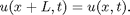
The nature of solutions depends on the system size L and on the initial u(x,0).

L = system size: For L = 22 the system accomodates

basic wavelengths and appears "turbulent".

Reasonable time scale: the shortest periodic orbit is

Matlab function ksfmstp.m computes the solution of the Kuramoto-Sivashinsky equation using Exponential Time Difference Runge-Kutta 4th order method (ETDRK4)

N = number of complex Fourier modes, h = time step, nstp = # time steps

  N = 64;  L = 22;  h = 0.25;  nstp = 1000;
  a0 = zeros(N-2,1);  a0(1:4) = 0.6; % just some initial condition
  [tt, at] = ksfmstp(a0, L, h, nstp, 1);
  fig1 = figure('pos',[5 550 600 400],'color','w'); plot(tt,at,'.-');
  title('Solution of Kuramoto-Sivashinsky equation with L = 22: Fourier modes');
  xlabel('Time'); ylabel('Fourier modes');

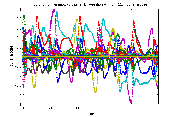
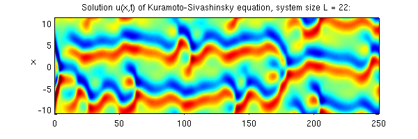
No insight is gained by staring at the Fourier modes. More helpful is the solution viewed in the space-time plot (x,t), with color code indicating the height of u(x,t). Go back to the u(x,t) representation by transforming the solution using function ksfm2real.m:

  [x, ut] = ksfm2real(at, L);
  fig2 = figure('pos',[5 270 600 200],'color','w');
  pcolor(tt,x,ut); shading interp; caxis([-3 3]);
  title('Solution u(x,t) of Kuramoto-Sivashinsky equation, system size L = 22:');
  xlabel('Time'); ylabel('x','rotat',0);

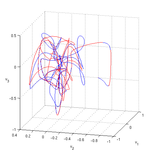
The solution can be also viewed in the state space projections. Here we span a 3-dimensional subspace by stability eigenvectors of the E2 equilibrium point (2-wavelength steady state).

  load('ks22statespace','v');  % v - subspace orthonormal vectors
  av = v'*at;  % projection of solution onto the subspace
  fig3 = figure('pos',[610 450 500 500],'color','w');
  plot3(av(1,:),av(2,:),av(3,:),'b'); grid on;
  xlabel('v_1'); ylabel('v_2'); zlabel('v_3','rotat',0); view(-75,15);

Sensitive dependence on initial condition

Start another solution with a nearby initial condition and see how it diverges from the first one. You might use such simulation as a starting point for evaluation of theleading Lyapunov exponent.

  a1 = a0;  a1(1) = a1(1) + 1e-3;
  [tt, at1] = ksfmstp(a1, L, h, nstp, 1);  av1 = v'*at1;
  figure(fig3); hold on;
  plot3(av1(1,:),av1(2,:),av1(3,:),'r');

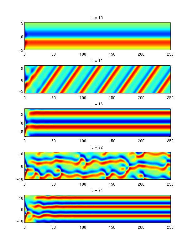
Dependence of KS solutions on L

  LL = [10 12 16 22 24];
  fig4 = figure('pos',[500 100 600 800],'color','w');
  for ii = 1:length(LL);
    [tt, at] = ksfmstp(a0, LL(ii), h, nstp, 1);
    [x, ut] = ksfm2real(at, LL(ii));
    subplot(length(LL),1,ii);
    pcolor(tt,x,ut); shading interp; caxis([-3 3]);
    title(['L = ' num2str(LL(ii))]);
  end

The equilibria and travelling waves of KS equation with L = 22

File ks22equilibria contains information about equilibria and travelling waves of KS equation with L = 22. The data are organized as arrays of structures: eq for equilibria and tw for travelling waves:

eq(k).a - coordinates of equilibria in Fourier space, k = 1,2,3 (there are three equilibria).

eq(k).eig - eigenvalues of the Jacobian of the flow at equilibria

eq(k).evec - corresponding eigenvectors

tw(k).a - coordinates of travelling waves in Fourier space, k = 1,2

tw(k).c - speeds of the travelling waves

tw(k).eig and tw(k).evec - as for equilibria, except that the Jacobian is calculated in the frame travelling with the wave (with speed c).

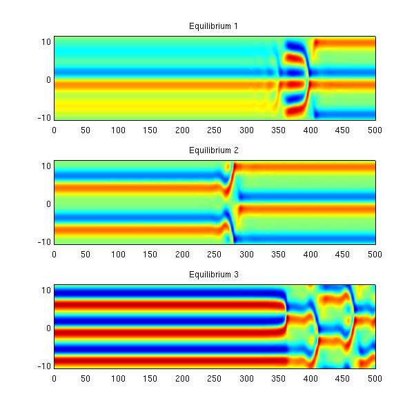
Here we plot evolution of solutions starting at equilibria. Since the equilibria are unstable and the initial conditions contain round-off errors, the solutions eventually move away from the equilibria.

  load ks22equilibria;  h = 0.25; nstp = 2000;
  fig5 = figure('pos',[700 200 600 600],'color','w');
  for k = 1:3,  a0 = eq(k).a;
    [tt, at] = ksfmstp(a0, L, h, nstp, 2); [x, ut] = ksfm2real(at, L);
    subplot(3,1,k);
    pcolor(tt,x,ut); shading interp; caxis([-3 3]);
    title(['Equilibrium ' num2str(k)]);
  end

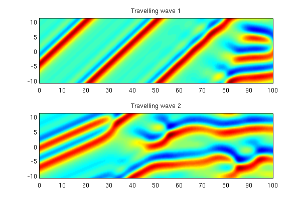
Solutions starting from the travelling waves can be plotted in a similar way.

  nstp = 400;
  fig5 = figure('pos',[700 300 600 400],'color','w');
  for k = 1:2,  a0 = tw(k).a;
    [tt, at] = ksfmstp(a0, L, h, nstp, 1);  [x, ut] = ksfm2real(at, L);
    subplot(2,1,k);
    pcolor(tt,x,ut); shading interp; caxis([-3 3]);
    title(['Travelling wave ' num2str(k)]);
  end

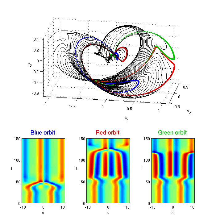
Plotting unstable manifolds of equilibria

Here's an example of how to visualize the unstable manifold of Equilibrium 2 in the state subspace spanned by selected eigenvectors.

Equilibrum 2 has a pair of complex conjugate eigenvalues:

An orbit starting close to the equilibrium will spiral out with a period

In order to trace out the unstable manifold, we start with a set of initial conditions

where v_1 is a unit vector parallel to the real part of the unstable eigenvector.

Coordinate axes (v_1,v_2,v_3) are constructed by Gram-Schmidt orhonormalization of (Re e_1, Im e_1, Re e_7), where e_j are the eigenvectors of the 2-wave equilibrium.

  clear; load ks22equilibria;  k = 2;  h = 0.1;  tend = 150;  av = [];
  ere = real(eq(k).eig(1));  period = 2*pi/imag(eq(k).eig(1));
  v = gsorth([real(eq(k).evec(:,1)) imag(eq(k).evec(:,1)) real(eq(k).evec(:,7))]);
  for delta = [0:0.1:ere*period 2.7 0.24 0.254],
    a0 = eq(k).a + 1e-4.*exp(delta).*v(:,2);
    [tt, at] = ksfmstp(a0, L, h, tend/h, 2); av = [av; v'*at];
    if delta == 2.7, at1 = at; end
    if delta == 0.24, at2 = at; end
  end,
  fig7 = figure('pos',[100 200 700 700],'color','w');
  ax1 = axes('pos',[0.2 0.46 0.63 0.52]);
    plot3(av(1:3:end-8,:)',av(2:3:end-7,:)',av(3:3:end-6,:)','k-');
    hold on; grid on; axis equal; view(10,20);
    plot3(av(end-8,:)',av(end-7,:)',av(end-6,:)','b.-');
    plot3(av(end-5,:)',av(end-4,:)',av(end-3,:)','r.-');
    plot3(av(end-2,:)',av(end-1,:)',av(end,:)','.-','color',[0 .8 0]);
    xlabel('v_1'); ylabel('v_2'); zlabel('v_3','rotat',0);
  ax2 = axes('pos',[0.10 0.06 0.20 0.30]);
    [x, uu] = ksfm2real(at1, L); pcolor(x,tt,uu'); caxis([-3 3]);
    shading flat; xlabel('x'); ylabel('t','rotat',0);
    ht = title('Blue orbit');  set(ht,'color','b','fontsize',15);
  ax3 = axes('pos',[0.40 0.06 0.20 0.30]);
    [x, uu] = ksfm2real(at2, L); pcolor(x,tt,uu'); caxis([-3 3]);
    shading flat; xlabel('x'); ylabel('t','rotat',0);
    ht = title('Red orbit');  set(ht,'color','r','fontsize',15);
  ax4 = axes('pos',[0.70 0.06 0.20 0.30]);
    [x, uu] = ksfm2real(at, L);  pcolor(x,tt,uu'); caxis([-3 3]);
    shading flat; xlabel('x'); ylabel('t','rotat',0);
    ht = title('Green orbit');  set(ht,'color',[0 .8 0],'fontsize',15);

Published with MATLAB® 7.2